Home / Statistical Tools / Distribution Fit/Calc / Distribution Fit / Understanding Distribution Fit Results
Understanding Distribution Fit Results
After using Specific Distribution Fitting or Auto-Fit Distribution Fitting, Quantum XL will display the results on a new worksheet in the active workbook. Quantum XL will create the following as part of the analysis.
- Graph of the probability density function (pdf)
- Probability out of spec, Cpk, and Cp (if spec limits are provided)
- Probability Plot
- Maximum Likelihood Estimates (MLE) of Parameters
- Goodness of Fit
- Descriptive Statistics
- Percentiles
Graph of the Probability Density Function (pdf)
The pdf describes the relative likelihood that the data will be a given value. If you supplied an Upper Spec Limit (USL) and/or Lower Spec Limit (LSL), then the area of the pdf outside of spec will be denoted in red.
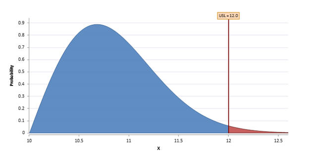
Probability Out of Spec, Cpk, and Cp
If spec limits (USL, LSL, or Both) were provided, then Quantum XL will calculate the probability of being out of spec and the Cpk statistics. In the example below, the Upper Spec Limit (USL) was defined but the Lower Spec Limit (LSL) was not. Quantum XL calculated the probability of being greater than the USL. Note that P(x>=12) can be expressed in percentage or defects per million (dpm). In this case, 1.39% of the distribution is greater than 12. To calculate dpm, multiple percent times 1 million or in this case 1.39%*1,000,000 = 13,881.1. The Cpk, Cp, CPU, and CPL statistics are calculated if possible.
Cpk requires either LSL, USL, or Both. Cp requires LSL and USL. CPL requires LSL. CPU requires USL. For the Normal (Gaussian) distribution, the reported Cpk is the Long Term. For all other distributions, see the topic Calculation of Cpk, CPL, and CPU for Non-Normal Data.
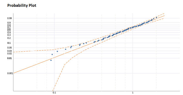
Probability Plot
The probability plot with the 95% confidence bounds provides a visual representation of the fit of the data. The X and Y Axis are linearized for the specific distribution. In general, data that falls along the center line is a good fit of the distribution. For the Normal distribution, the Confidence Bounds are calculated using Lilliefors method. For more information, see the following.
Stephens, M. A. "EDF Statistics for Goodness of Fit and Some Comparisons." Journal of the American Statistical Association 69.347 (1974): 730. Lilliefors, Hubert W. "On the Kolmogorov-Smirnov Test for Normality with Mean and Variance Unknown." Journal of the American Statistical Association 62.318 (1967): 399.
For other distributions, the calculation relies on the Hessian matrix using the partial derivatives. For more information, see the following.
Meeker, W. Q. and Escobar L. A., "Statistical Methods for Reliability Data", 1998, New York, Wiley
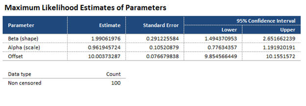
Maximum Likelihood Estimates of Parameters
Quantum XL provides text display of the parameters of the chosen distribution. The example below is for the three parameter Weibull distribution. For more information about calculation of these parameters, see Maximum Likelihood Estimation.
Goodness of Fit (Anderson Darling)
Quantum XL uses the Anderson Darling for all distributions. Note that the Anderson Darling p-value isn't available when your data has censored values. The three parameter Weibull is the only distribution with a threshold where the Anderson Darling p-value is available.
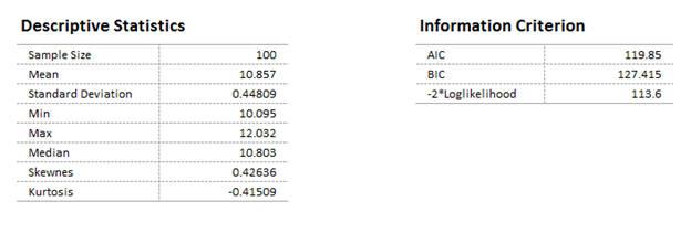
Descriptive Statistics
Quantum XL displays the descriptive statistics for the dataset along with the Information Criteria.
Percentiles
Quantum XL provides text results for various percentiles. See the Probability Plot for a graphical representation.
Hazard Plot
Plot of the instantaneous failure rate.
Survival Plot
Plot of the percentage of the population surviving vs. time. It is also 1-CDF(x) where CDF is the cumulative distribution function.
See Also
- Named Distribution Fitting (without Auto-Fit)
- Calculation of Cpk, CPL, and CPU for Non-Normal Data
- Maximum Likelihood Estimates
- AIC and BIC
- Johnson Transformation
- 2-Parameter Normal
- 1-Parameter Exponential
- 2-Parameter Exponential
- 2-Parameter Logistic
- 2-Parameter LogLogistic
- 3-Parameter LogLogistic
- 2-Parameter LogNormal
- 3-Parameter LogNormal
- 2-Parameter Weibull
- 3-Parameter Weibull
- 2-Parameter Gumbel/Smallest Extreme Value (SEV)