Home / Monte Carlo / Analyzing The Model / Optimize (Parameter Design)
Optimize (Parameter Design)
From Excel click...
QXL Monte Carlo Tab > Optimize
The optimizer can be used to reduce the defects per million of all the outputs simultaneously (Standard Mode) or to run an optimization on other statistics (e.g., mean, standard deviation, median, percentiles, etc.).
Reduce DPM -- Standard mode
The purpose of Parameter Design in Standard Mode is to reduce the defects per million (dpm) by finding the optimal input location parameter. The optimization is a true stochastic (with variation) process. A simplified version of the process that is used for optimization is shown below.
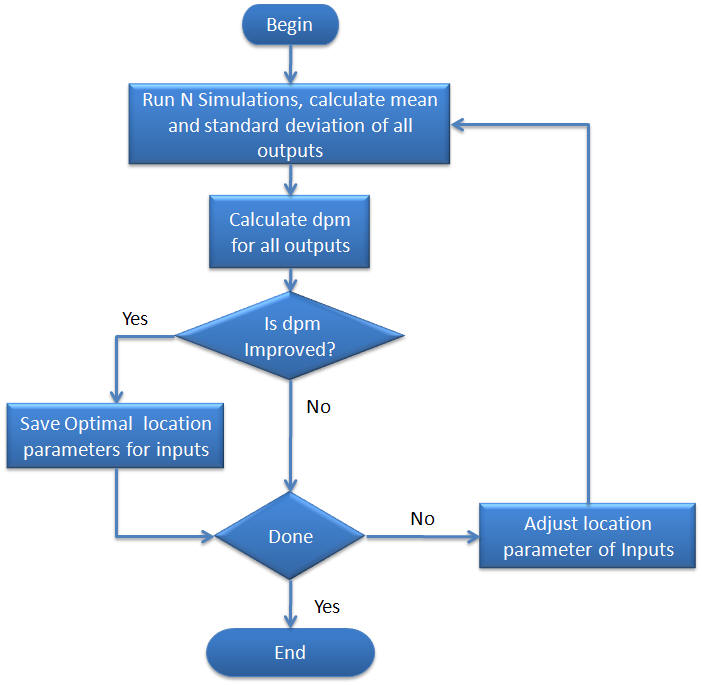
The objective function of the optimization is a calculated value of defects per million (dpm). In order to calculate the dpm, N Monte Carlo simulations are performed. The data resulting from the simulations is then used to calculate the dpm (see dpm vs. # out of spec for more information on how dpm can be calculated).
Setup Optimization
Quantum XL will need a variety of information to successfully run an optimization: optimization objective, optimization constraints, the range of valid inputs, and the type of dpm for each of the outputs.
Step #1: Optimization Objectives
At this step you should specify the Objective that you would like to optimize.
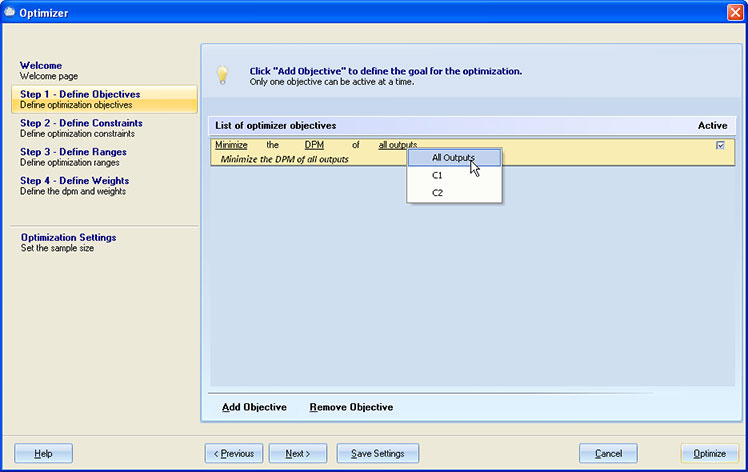
Use theAdd Objectivebutton to add a new objective. The objective row shows elements that can be modified by underlining them. If you click on them, a list of available options will pop up. The objective is made up of the Objective Goal, Objective Statistic, and Output.
-
Objective Goal: You can choose to Minimize, Maximize or Set the target for specified statistics of a specified output.
-
Objective Statistic: Specify the desired statistic you want to minimize or maximize. There is a long list of statistics from which you can choose, like Mean, Median, Probability, etc.
-
Output: Select the output you are setting the objective for. If the model supports optimization to minimize the dpm for all outputs, the 'All outputs' option will be available in this group. The following conditions must be met to enable the 'All outputs' option: two or more outputs must have specification limits defined; the Objective Goal must be 'Minimize'; and the Objective Statistic must be 'DPM'.
The first time you start the optimization, it will set the default Objective.
-
If the model has two or more outputs with defined specification limits, the default will be to minimize the dpm for all outputs.
-
If only one output has defined specification limits, the default Objective will be to minimize the dpm for that output.
-
If there are no outputs with defined specification limits, the Optimizer will not set the default Objective.
There can be only one objective active for the optimization. However, you can define multiple objectives, save them by clicking the Save Settings button, and activate them one at a time.
Step #2: Optimization Constraints
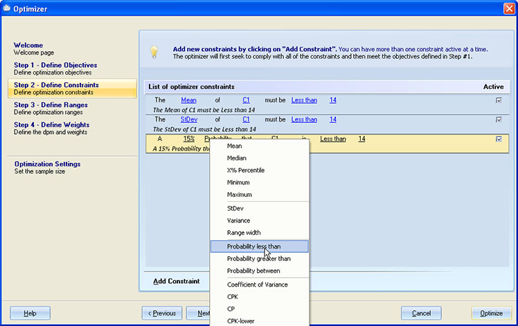
Use the Add Constraints button to add a new constraint. The constraints row has elements that can be modified. These elements are underlined. If you click on them, a list of available options will pop up. A constraint is made up of Constraint Statistic, Output, and Constraint Metric.
-
Constraint Statistic: There is a long list of statistics from which you can choose, like Mean, Median, Probability, etc.
-
Constraint Output:Select the output you are setting the constraint for.
-
Constraint Metric: The metric can be 'Less than', 'Greater than', and 'Between'.
During optimization, the optimizer will check all constraints and it will change inputs in such a way so that all constraints are met. Therefore, you cannot define constraints that are not compatible. I.e., you cannot define two constraints like this:
-
The Mean of MyOutput1 must be less than 10, and
-
The Mean of MyOutput1 must be greater than 20
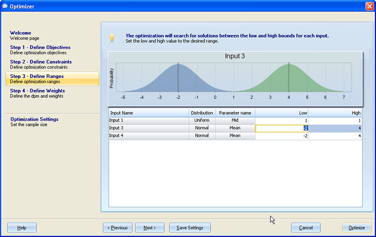
Step #3: Define the lows and highs for the input variable
This step is available in both Advanced and Standard modes.
When you first initiate Parameter Design, you will be given the opportunity to define the lows and highs for each input location parameter. In the example below, "Input 3" is Normally Distributed. The location parameter for the Normal Distribution is the mean, and so in the column entitled "Parameter Name" the word "Mean" is displayed for Input 3. The current values for Low and High are --2 and 4 respectively. This will allow the optimizer to shift the mean anywhere from --2 to 4 when trying to reduce the dpm. The other parameters of the distribution will not change during the optimization. Therefore, in this example, the standard deviation will not change during the optimization.
The location parameter for each distribution will be displayed in the distribution column. It should be noted that while Quantum XL will optimize based upon any ranges specified for the location parameter, it may not be possible for you to change the location parameter in your actual design/process. You must take care that you are able to make the changes in the distribution.
-
Normal Distribution: The low and high values define the acceptable low and high values for the mean. The standard deviation does not change during parameter design.
-
Exponential Distribution: The low and high values define the acceptable low and high value for lambda.
-
Uniform Distribution: The low and high values define the acceptable low and high values for the mean. The mean of the uniform distribution is equal to the (Lower Bound + Upper Bound)/2. The standard deviation of the uniform distribution does not change during parameter design.
-
Empirical Data Distribution: The empirical data distribution is fixed; it does not change during parameter design.
-
Triangular Distribution: During optimization, the mode is changed within the specified range while the minimum and maximum are changed to reflect the original shape of the distribution.
See Supported Distributions for more information on optimization parameters for other distributions.
Inputs that were marked as 'Noise Inputs', will not be included in this screen. Their optimization Low and High will be adjusted so that the location parameter does not change during the optimization.
Step #4: Define the type dpm and weights for each output response
This step is available in Standard mode.
For each output, you can designate the type dpm and weight. The weights are only important if you have more than one output. The goal of parameter design is to maximize the total weights.
The weights are computed as Wi*((1,000,000-dpmi)/1,000,000) where Wiis the weight for that output. For example, if you have two outputs with the following weights and dpm:
| Weight | dpm | |
|---|---|---|
| Output #1 | 100 | 500,000 |
| Output #2 | 50 | 100,000 |
The total weight will be:
Total Weight = 100((1,000,000-500,000)/1,000,000) + 50((1,000,000-100,000)/1,000,000) = 100.5 + 50.9 = 50+45 = 95.
It should be noted that you (the user) define the weight for each output and Quantum XL calculates the dpm during the optimization procedure. In this example, the user has assigned a total of 150 weight points, 100 for Output #1 and 50 for Output #2. The best possible total weight would be 150 and would occur when the dpm for each of the outputs is equal to zero.
| Weight | dpm | |
|---|---|---|
| Output #1 | 100 | 0 |
| Output #2 | 50 | 0 |
Total Weight = 100((1,000,000-0)/1,000,000) + 50((1,000,000-0)/1,000,000) = 1001 + 501 = 100+50 = 150.
The worst possible solution would be when Output 1 and Output 2 both have 1,000,000 dpm.
| Weight | dpm | |
|---|---|---|
| Output #1 | 100 | 1,000,000 |
| Output #2 | 50 | 1,000,000 |
Total Weight = 100((1,000,000-1,000,000)/1,000,000) + 50((1,000,000-1,000,000)/1,000,000) = 1000 + 100 = 0+0 = 0.
Therefore, the Total Weight is always bound between 0 (worst possible solution) and the sum of the weight points (best possible solution).
If you only have one output, the weight is not important. The purpose of "weighting" an output is to increase its importance relative to the other outputs. In the example above, Output #1 is twice as important as Output #2.
After this step, the Optimization Display will appear. It displays the optimization progress. Inputs are located at the left pane and the outputs on the right.
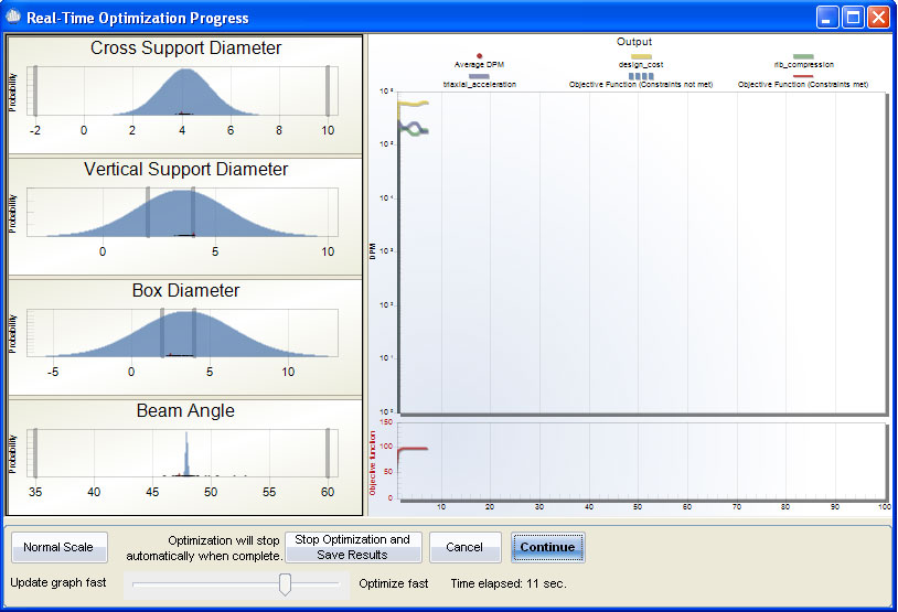
Display
On the left side, the current optimal input distributions are displayed. In the example above, there are four inputs which are all normally distributed. The grey vertical lines indicate the minimum and maximum the mean can be shifted during optimization (defined in step #1). The small black dots on the horizontal axis display where the optimizer is currently searching for a new optimal mean for that input.
On the right side of the display you will see two plots. The top plot displays the current dpm for each of the outputs and an Average dpm for all of the outputs. As the optimizer finds better solutions, the values of these dpms will reduce and become closer and closer to zero.
The plot on the bottom right is the objective function. The objective function is the sum of the total weight points (see explanation above of Wi*((1,000,000-dpmi)/1,000,000)).
Stop Optimization and Save Results-- Press to stop the optimization and have the location parameters written back to the model sheet.
Cancel-- Stops the optimization.
Continue/Pause-- Pauses and then restarts the optimization.
Update speed slider-- Move to the right to update the display less frequently (faster optimization).
Normal Scale / Log Scale-- Switch between Normal and Log scale on the outputs plot.
The optimizer will run until it can no longer improve the process or until the user stops the process.
Some special considerations regarding Optimization Display
-
If the optimization goal is to Minimize DPM for all outputs, the following lines will be plotted on the outputs section: dpm line for each output; average dpm line; and objective function.
-
For optimization other than Minimize DPM for all outputs, only one line will be plotted on the outputs section.
-
The objective line on the outputs section can be a dotted line (meaning Constraints were not met yet), or a solid line (there are no Constraints, or all Constraints are met).
-
If there are too many inputs for the optimization display to handle, the optimizer will list all inputs in the List Box, instead of plotting them.
-
If there are too many outputs (this can happen only if the goal is to Minimize DPM for all outputs), the optimizer will plot only the average dpm and the objective function.
-
Noise Inputs are not plotted.