Home / Monte Carlo / Model Building / Supported Distributions
Monte Carlo Supported Distributions
Continuous Distributions
Discrete Distributions
Normal Distribution
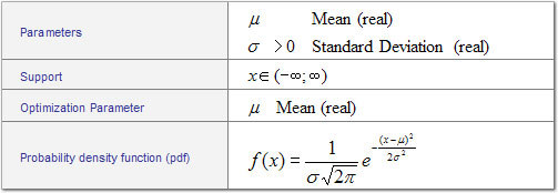
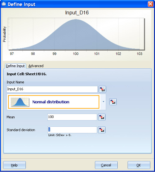
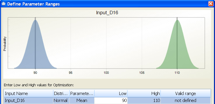
During optimization, the mean is changed within the specified range while the standard deviation is maintained at its defined level. For example, if you define an input as N(100,1) and then during optimization enter a range of 90 to 110, the optimizer is able to set the mean for this input to any mean value between 90 and 110 while maintaining the standard deviation of 1. In the diagram below, the blue curve represents the smallest mean the optimizer will try and the green curve represents the largest mean the optimizer will try.
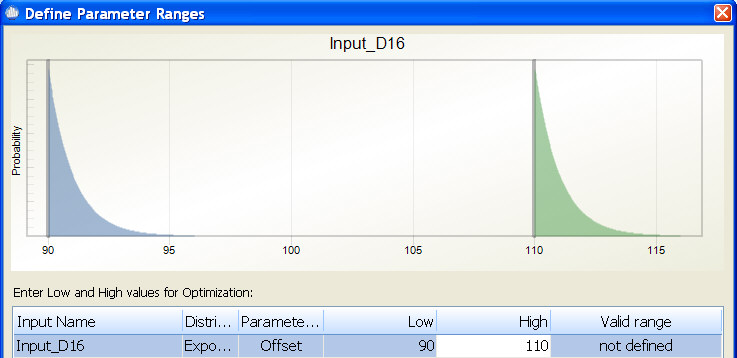
Exponential Distribution
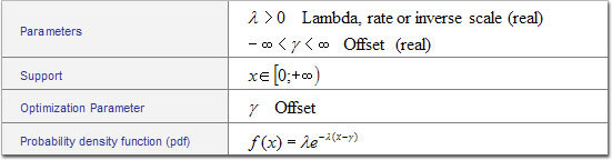
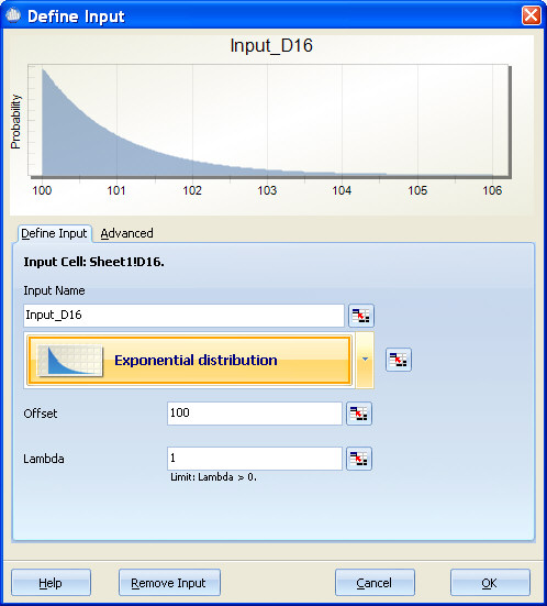
During optimization, the offset is changed within the specified range while lambda is maintained at its defined level. For example, if you define an input as exponential with an offset=100 and lambda=1, and then during optimization enter low=90 and high=110, the optimizer is able to set the offset for this input to any offset value between 90 and 110 while maintaining the lambda=1. In the diagram below, the blue curve represents the smallest lambda the optimizer will try and the green curve represents the largest lambda the optimizer will try.
Uniform Distribution
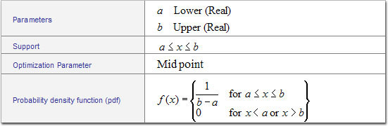
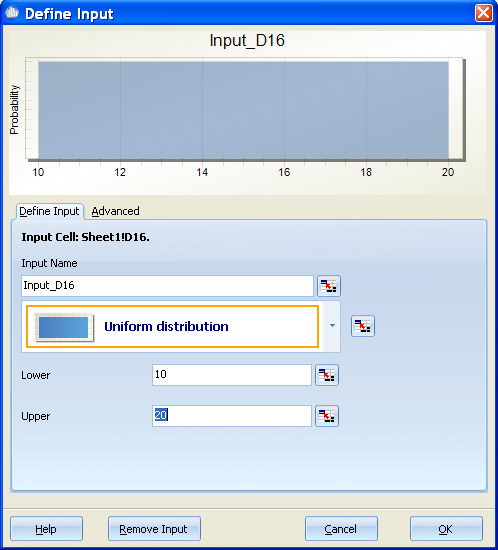
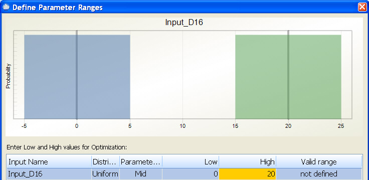
During optimization, the midpoint is changed within the specified range while the variation is maintained at its defined level. For example, if you define an input as Uniform with Lower=10 and Upper=20, the midpoint is calculated to be 15. If during optimization you enter low=0 and high=20, the optimizer is able to set the offset for this input to any offset value between 0 and 20 while maintaining the original range which is +/-5. This can be confusing since the midpoint is not one of the original parameters collected; however, if you defined the Uniform as having a lower=10 and upper=20, then this can also be thought of as 15 +/-5 or mid +/-5. During optimization, the mid value will change, but the +/-5 will not. In the diagram below, the blue curve represents the smallest midpoint that optimizer will try and the green curve represents the largest midpoint the optimizer will try.
Special considerations for the Uniform Distribution
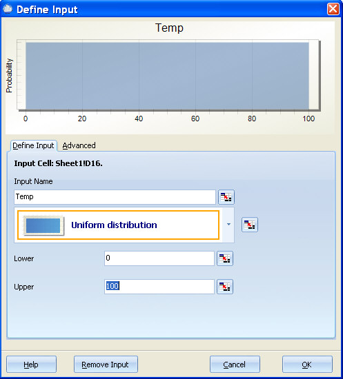
The most common use of the Uniform Distribution is to model noise variables. For example, if you expect your customer to use your product in temperatures ranging from 0 degrees to 100 degrees, you may model Temp as Uniform from 0 to 100 (see below)
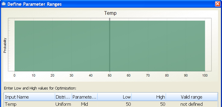
In this case, you would normally not want the optimizer to pick an optimal midpoint for the temperature. By default, Quantum XL will set the low and high for the optimizer in a way such that the midpoint will not change during optimization. For this example, the temperature is Uniform from 0 to 100, so the midpoint is 50. Quantum XL will automatically set the low and high for optimization equal to 50 so that the midpoint will not change. The result is that the optimizer will always generate random numbers from 0 to 100 during optimization. The blue and green curves, which represent the smallest and largest mid points that can be used in optimization, overlap as no change is allowed (see below).
Triangular Distribution
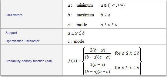
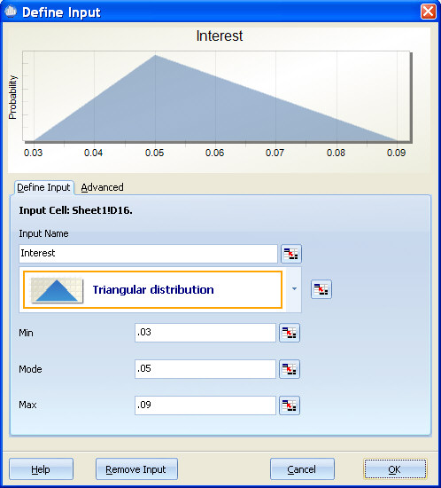
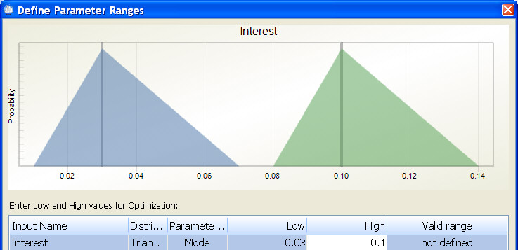
During optimization, the mode is changed within the specified range while the minimum and maximum are changed to reflect the original shape of the distribution. For example, if you define an input as Triangular with Min=.03, Mode=.05, and Max=.09, and then during optimization enter low=.03 and high=.1, the optimizer is able to set the mode for this input to any offset value between .03 and .1 while maintaining the original shape of the distribution. In the diagram below, the blue curve represents the smallest mode the optimizer will try and the green curve represents the largest mode the optimizer will try.
Log-Normal Distribution
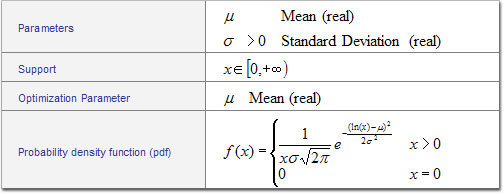
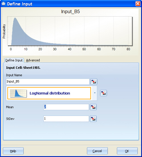
Optimization Notes: See Normal Distribution
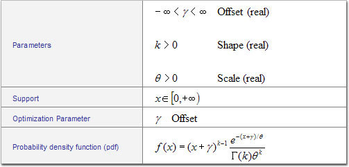
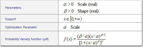
Weibull Distribution
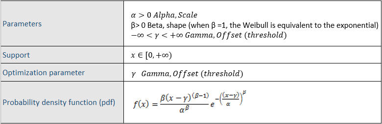
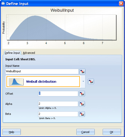
Special Notes: Different text books and articles use the parameters of the Weibull distribution differently. Quantum XL uses the same probability density function (pdf) as Excel. You should exercise care if you obtained your estimates for alpha and beta from another software application or Weibull paper. If the pdf you are using doesn't match the one used by Quantum XL, then usually you can convert your alpha and beta with some basic math. For example, try reversing alpha and beta or try inverting alpha and beta. While the use of alpha and beta are not standardized, the form of the Weibull distribution is usually the same.
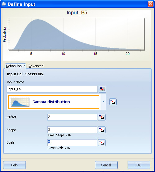
Gamma Distribution
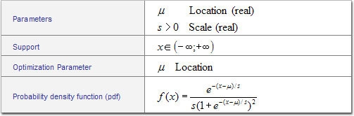
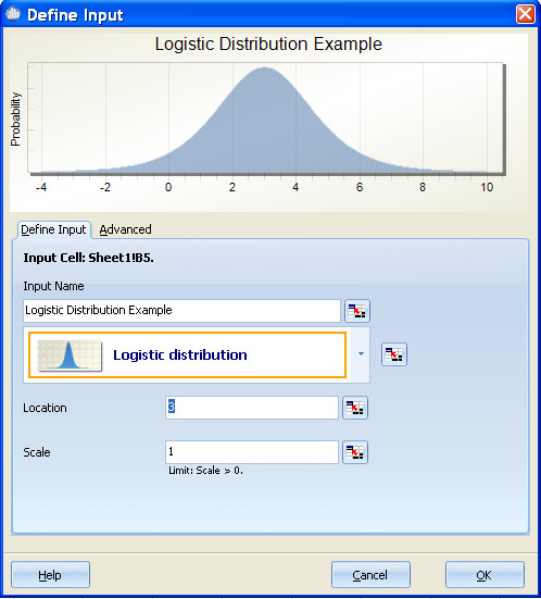
Logistic Distribution
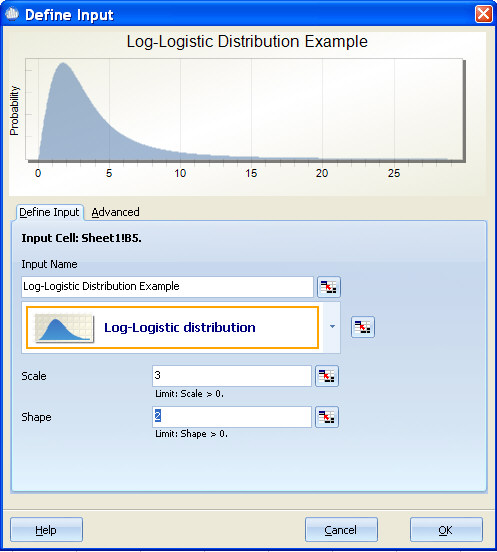
Log-Logistic Distribution
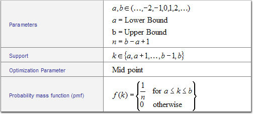
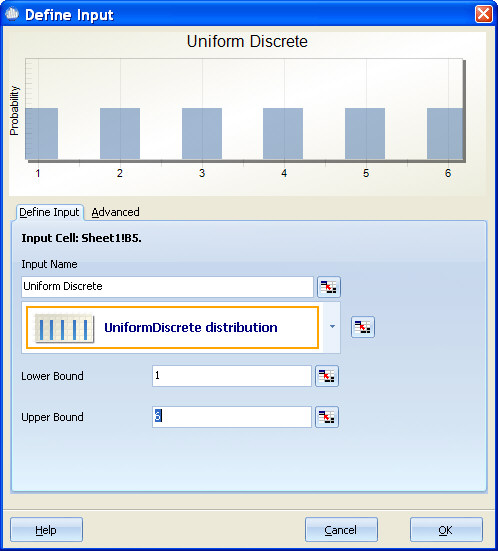
Uniform (Discrete) Distribution
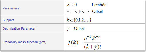
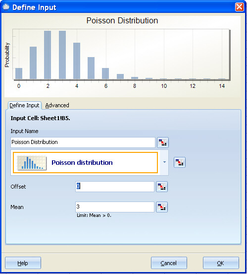
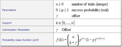
Poisson Distribution
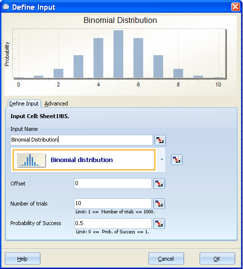
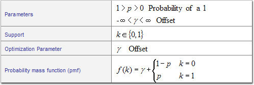
Binomial Distribution
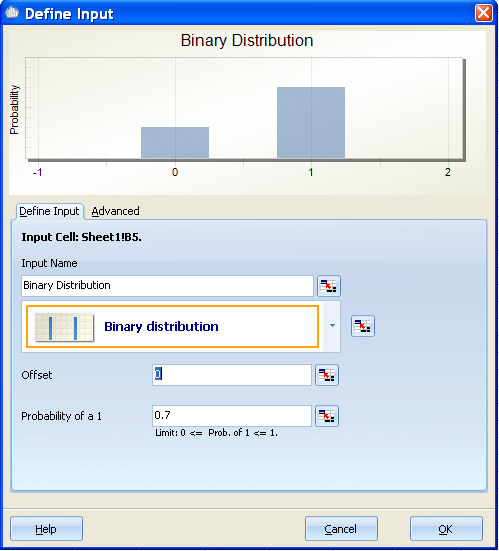
Binary Distribution
Special Notes: The Binary Distribution serves to model a binary variable. A typical use would be to model a qualitative noise variable. An example would be a model for fuel efficiency that includes two different Gas Types. Assume that you have a function in the form Fuel Efficiency=f(Gas Type, other variables), where Gas Type 0=Brand A and Gas Type 1=Brand B. You can use the Binary Distribution to generate 0 and 1 to mimic the variation that you would experience in using the two different brands.
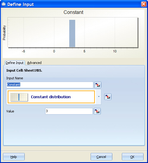
Constant Distribution
Parameters: Constant
Optimization Parameter: Constant
Special Notes: The Constant Distribution isn't a distribution at all. It is provided for values that will not change during a simulation. The advantages of using the constant distribution over a scalar value in a spreadsheet is the ability to optimize on the value of the constant. Using the constant is the same as modeling an input as Normal with a standard deviation of zero.